Why being wrong is better than being right (if you’re a model).
When estimating the relationship between two variables we want this estimate to be as close to the true relationship as possible, right? Wrong. Often an estimate that is wrong is better than one that is right.
OK, I’ll admit it: I like models. I especially like models because they are predictable and simple. And I like my models to be wrong. This may sound counterintuitive, but when making predictions a model that is wrong is often better. Let me show you why.
Suppose we set out to discover the relationship between age and a certain cognitive ability. We conduct an experiment in which participants of different ages perform a cognitive task measuring this ability. The data, age on the x-axis and ability on the y-axis, are plotted in Figure 1. The gray Xs are the observed data; the red circles show the actual shape of the relationship. Our task is thus to discover the relationship between ability and age. Or, more formally, our task is to find the function f that relates age and ability:
ability=f(age)+ε (1)
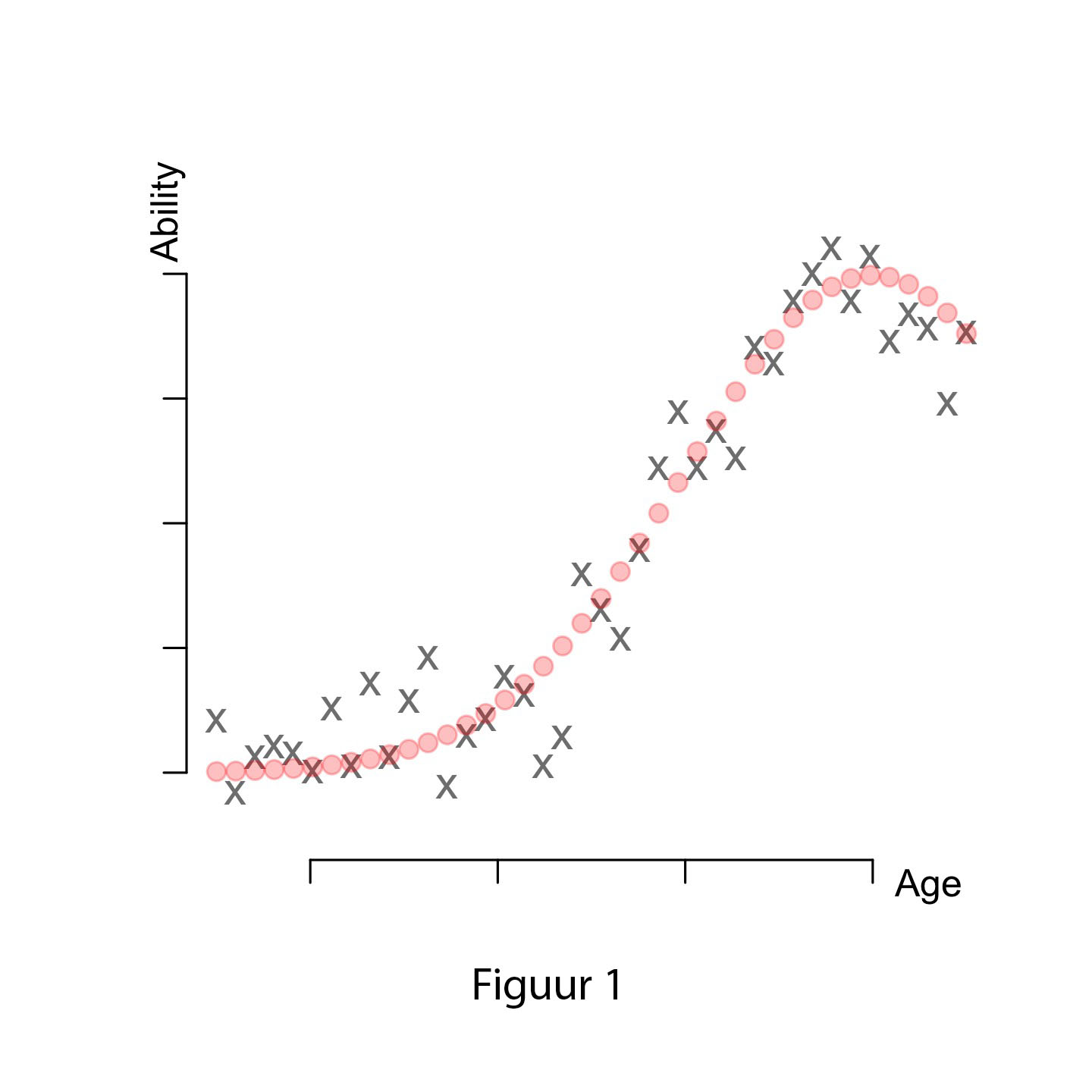
In this equation, f is the true function that defines the shape of this relationship (red circles), and ε is the error term (differences between red circles and gray Xs). Error in this case could come from many sources. It could be measurement error due to the task. It could be error due to participants’ characteristics (e.g. mood, concentration). It could even be error from another confounding variable that influences the relationship (e.g. people with higher intelligence score higher on our ability task). Whatever the source of the error, we don’t know how big this error is: we only know the gray Xs. That is why we call ε irreducible error.
So the data we observed contain the true relationship and some unidentifiable error. How can we now best go about finding this relationship? The most common way is to use a statistical model, like this one:
predicted ability=f ̂ (age) (2)
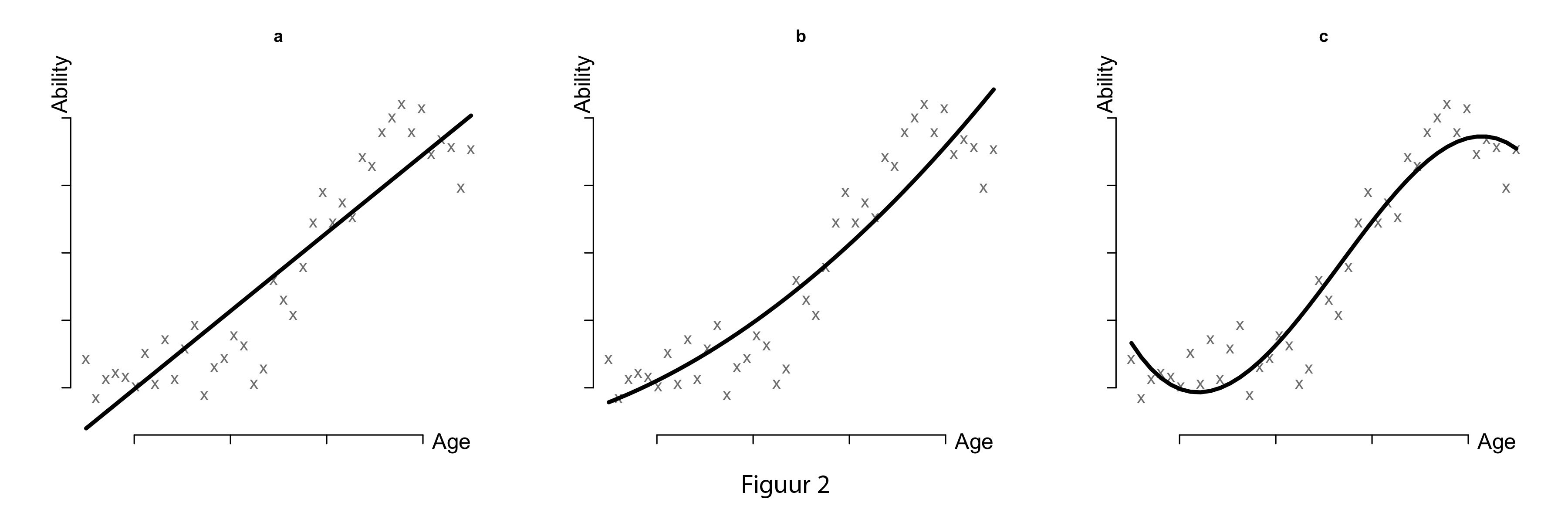
In this formula, f ̂ is our prediction for the shape of the relationship and predicted ability contains the estimated ability scores. But how do we decide what shape of f ̂ is our best guess for the true relationship? The easiest way to do this is to fit different models and see which models make the best predictions of ability. This is shown in Figures 2a through e. The first three Figures (2a-c) show a linear model, a quadratic model, and a cubic model. With each step in the model we use a more complex function for f ̂ (with more parameters), and with each step we see that the fit of the model increases (the line fits the observed points better).
We could even go a step further and fit even more complex models. Figures 3a-b show two LOESS models that use a more complex shape function, the last model being the most complex of all. We see that fit goes up again, until we have even completely reduced the error: the model fits perfectly!
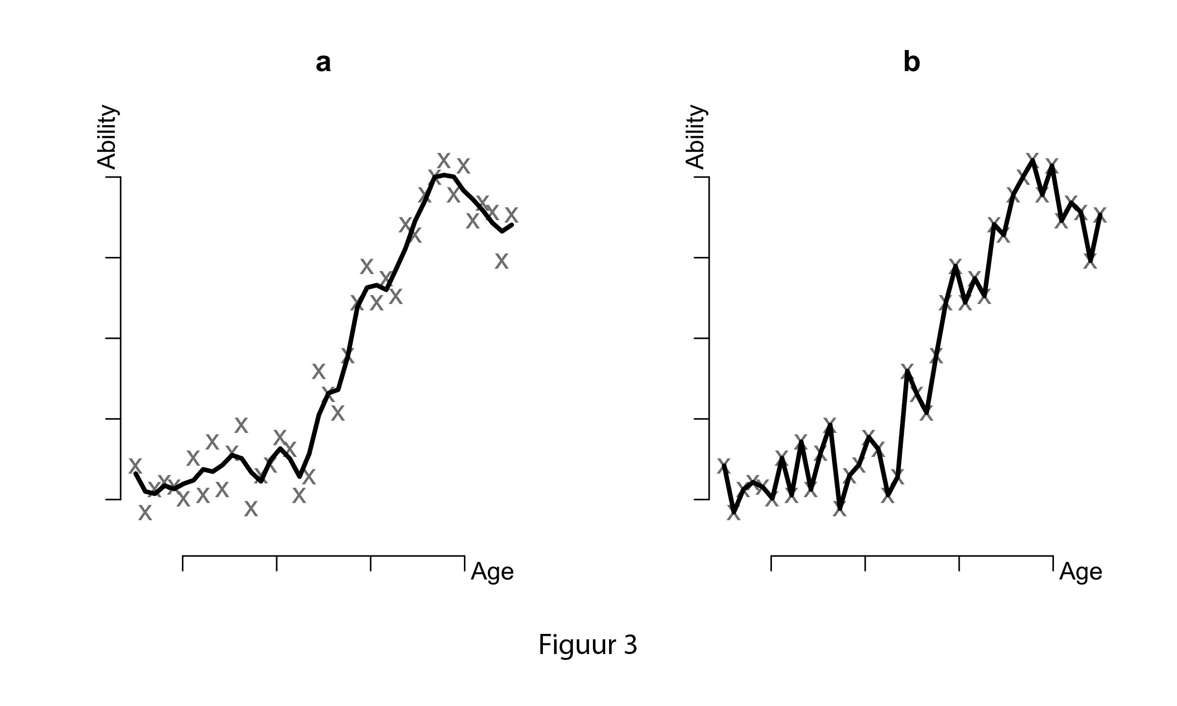
If you were in charge of analysis and if I were to ask you which model you would choose, my guess is that you wouldn’t opt for the LOESS models. You would probably choose one of the first three models. But why? Clearly, these models fit less well than our LOESS model, so why are we still opting for a model that contains more error? Your answer may have something to do with interpretability. While interpretability is a valid reason - we have to write down a description of the shape somewhere, after all - there is another reason why we (should) opt for a more ‘wrong’ model.
The reason has to do with bias and variance. To understand bias and variance we have to look at what happens when we fit increasingly complex models. With increased model complexity our error in predicting the data decrease. With this decrease in error we also decrease bias. Bias is defined as the difference between the shape of the true relationship f and the relationship we estimate from the data. So the more closely a model follows the data points, the closer we are (on average) to the true shape, and the smaller our bias is.
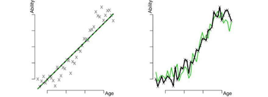
But what happens to our irreducible errors? As the complexity of the model increases, our estimated shape relies more and more on these errors. To see this, imagine what would happen to our estimates of model 2a if we did the experiment again and fitted this model to these new data. Would our estimates differ? They probably would to some degree, but not very much. This is shown in Figure 4a. Our new model estimates (black line) do not differ much from the estimates in our original model (green dotted line). Now imagine what would happen to the estimates of the most complex model (3b). They would probably differ to a greater extent in the new dataset, as these estimates will closely follow our new data points. This is shown in Figure 4b. The estimates from our new dataset (black line) will differ substantially from our original estimates (green line). Actually, with each new dataset, predictions from a complex model will vary to a greater extent than predictions from a simple model. In other words, with increased model complexity comes increased variance.
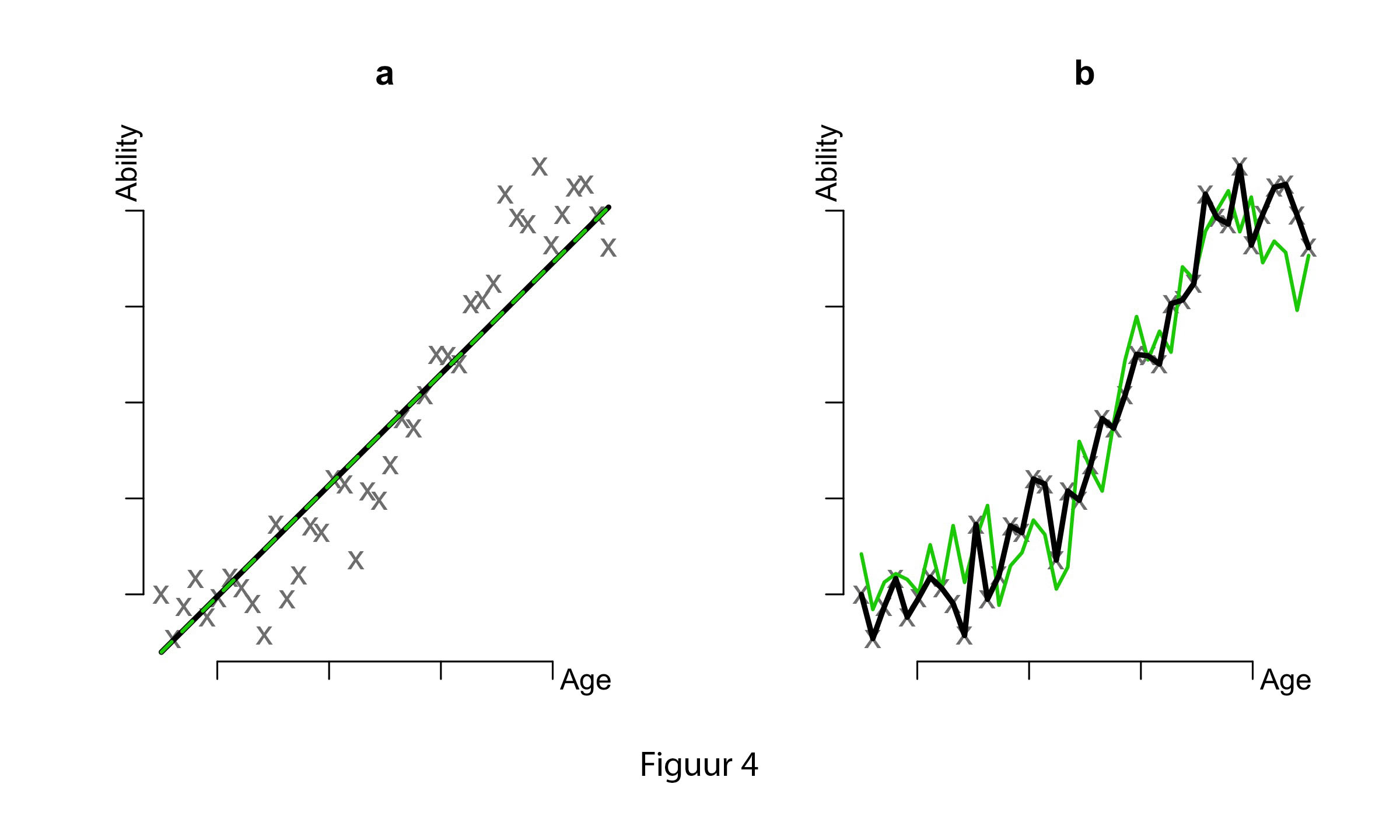
Figure 5 shows the relationship between bias and variance. On the x-axis is model complexity: left are simple models, right are more complex models. The y-axis indicates the total error, or how ‘wrong’ we are overall. As we can see, when we have a simple model, we have a high total error, containing mostly bias and little variance. Estimates are biased but stable across new datasets. If we opt for more complex models our total error will consist more of variance than of bias. Our predictions are less biased, but will vary substantially across new datasets.
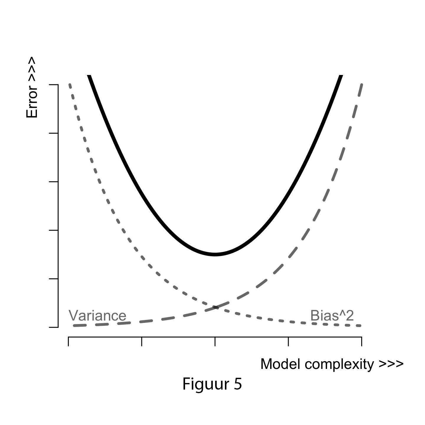
This leads us back to the question of why being wrong is better then being right. If we want to make predictions that generalize across new datasets, we can better choose a simple model. Complex models are less wrong overall, but predictions will vary substantially. So if you want your predictions to be right: “let thy model be wrong.”
References:


